Welcome to Probability

We will try to cover the fundamentals of probability. This is useful to quantify uncertainty and describe random events and outcomes.

Probability allows us to measure uncertainty. This is essential in many different industries, such as meteorology, medicine, sports, insurances, and countless more.

Probability is a branch of mathematics that allows us to quantify uncertainty. In our daily lives, we often use probability to make decisions, even without thinking about it.

Set Theory is a branch of mathematics based around the concept of sets. In simple terms, a set is a collection of things. For example, we can use a set to represent items in a backpack. We might have:

backpack = {'laptop', 'notebook', 'pencil', 'lunchbox'}

Notationally, mathematicians often represent sets with curly braces. Sets also follow two key rules:

• Each element in a set is distinct.
• The elements in a set are in no particular order.

  {1, 2, 3} = {3, 2, 1}

Experiments and Sample Spaces

In probability, an experiment is something that produces observation(s) with some level of uncertainty. A sample point is a single possible outcome of an experiment. Finally, a sample space is the set of all possible sample points for an experiment.

For example, suppose that we run an experiment where we flip a coin twice and record whether each flip results in heads or tails. There are four sample points in this experiment:

• (HH),
• (HT),
• (TH),
• (TT).

We can write the full sample space for this experiment as follows:

sample_space = {'HH', 'HT', 'TH', 'TT'}

Suppose we are interested in the probability of one specific outcome: HH. A specific outcome (or set of outcomes) is known as an event and is a subset of the sample space. Three events we might look at in this sample space are:

• Getting Two Heads (HH)
• Getting Two Tails (TT)
• Getting Both a Heads and a Tails (HT or TH)

The frequentist definition of probability is as follows:

Okay, we have flipped two coins 1000 times. Here are each of the outcomes and the number of times we observed each one:

• (HH) - 252
• (TT) - 247
• (HT) - 256
• (TH) - 245

To calculate the esimated probability of any one outcome, we use the following formula:

P(E) = (Number of times E occurs) / (Total number of trials)

so in our scenarios

P(HH) = 252 / 1000 = 0.252

Law of Large Numbers

We can't repeat our random experiment an inifinite amount of times. However, we can still flip both coins a large number of times. As we flip both coins more and more, the observed proportion of times each event occurs will converge to its true probability. This is the Law of Large Numbers.

Random variables

A random variable is, in its simple form, a function. In probability, we often use random variables to represent random events. For example, we could use a random variable to represent the outcome of a die roll: any number between one and six.

Random variable must be numeric, meaning they always take on a number rather than a characteristic or quality. If we want to use a random variable to represent an event with non-numeric outcomes, we can choose numbers to represent those outcomes. For example, we could represent a coin flip as a random variable by assigning heads a value of 1 and tails a value of 0.

The following code simulates the outcome of rolling a fair die twice using np.random.choice():

import numpy as np

# 7 is not included in the range function
die_6 = range(1, 7)

rolls = np.random.choice(die_6, size = 2, replace = True)

print(rolls)

DISCRETE RANDOM VARIABLES

A discrete random variable is a random variable that can take on a finite number of values. For example, the number of heads in three coin flips is a discrete random variable. It can take on the values 0, 1, 2, or 3. Discrete random variables are also common when observing counting events, such as how many people entered a store on a randomly selected day. In this case, the values are countable in that they are limited to whole numbers (we can't observe half of a person).

CONTINUOUS RANDOM VARIABLES

A continuous random variable is a random variable that can take on an infinite number of values. For example, the weight of a salmon is a continuous random variable. It can take on any value between 0 and infinity. Continuous random variables are common when observing measurements, such as weight, height, or time.

Probability Mass functions

A probability mass function (PMF) is a type of probability distribution that defines the probability of observing a particular value of a discrete random variable. For example, a PMF can be used to calculate the probability of rolling a three on a fair six-sided die.

There are certain kinds of random variables (and associated probability distributions) that are relevant for many different kinds of problems. These commonly used probability distributions have names and parameters that make them adaptable for different situations.

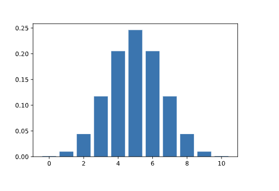
For example, suppose that we flip a fair coin some number of times and count the number of heads. The probability mass function that describes the likelihood of each possible outcome (eg., 0 heads, 1 head, 2 heads, etc.) is called the binomial distribution. The parameters for the binomial distribution are:

• n for the number of trials (eg., n = 10 if we flip a coin 10 times)
• p for the probability of success in each trial (probability of observing a particular outcome in each trial). In this example, p = 0.5 because the probability of observing heads on a fair coin flip is 0.5

If we flip a fair coin 10 times, we say that the number of observed heads follows a Binomial (n=10, p=0.5) distribution. The heights of the bars represent the probability of observing each possible outcome as calculated by the PMF.

Probability with Python

The binom.pmf() method from the scipy.stats library can be used to calculate the PMF of the binomial distribution at any value. This method takes 3 values:

• x: the value of interest
• n: the number of trials
• p: the probability of success

# import necessary library
import scipy.stats as stats

# st.binom.pmf(x, n, p)
print(stats.binom.pmf(6, 10, 0.5))

What if we want to find the probability of observing a range of values for a discrete random variable? One way we could do this is by adding up the probabilities of each individual value in the range.

We can use the same binom.pmf() method from the scipy.stats library to calculate the probability of observing a range of values. As mentioned in a previous exercise, the binom.pmf method takes 3 values:

• x: the value of interest
• n: the sample size
• p: the probability of success

import scipy.stats as stats

# calculating P(2-4 heads) = P(2 heads) + P(3 heads) + P(4 heads) for flipping a coin 10 times
print(stats.binom.pmf(2, n=10, p=.5) + stats.binom.pmf(3, n=10, p=.5) + stats.binom.pmf(4, n=10, p=.5))

Sampling from a Population

In statistics, we often want to learn about a large population. Since collecting data for an entire population is often impossible, researchers may use smaller sample of data to try to answer their questions.

Random Sampling in Python

The numpy.random package has several functions that we could use to simulate random sampling. In this example, we will use the function np.random.choice(), which generates a sample of some size a given array.

# you can use Jupyter Notebook
import numpy as np
import pandas as pd
import seaborn as sns
import matplotlib.pyplot as plt


population = pd.read_csv("salmon_population.csv")
population = np.array(population.Salmon_Weight)
pop_mean = round(np.mean(population),3)

## Plotting the Population Distribution
sns.histplot(population, stat='density')
plt.axvline(pop_mean,color='r',linestyle='dashed')
plt.title(f"Population Mean: {pop_mean}")
plt.xlabel("Weight (lbs)")
plt.show()

samp_size = 10
# Generate our random sample below
sample = np.random.choice(np.array(population), samp_size, replace = False)

### Define sample mean below

sample_mean = round(np.mean(sample),3)

sns.histplot(sample, stat='density')
plt.axvline(sample_mean,color='r',linestyle='dashed')
plt.title(F"Sample Mean: {sample_mean}")
plt.xlabel("Weight (lbs)")
plt.show()