Encoding Categorical Variable with Python

Categorical data is data that has more than one category. When working with that type of data we have two types, nominal and ordinal. Nominal data is data that has no particular order or hierarchy to it, and ordinal data is categorical data where the categories have order, but the differences between the categories are not important or unclear.

We will be working with a dataset of used cars for this article to truly understand and demonstrate how to work with categorical data. Let’s explore it and see what type of data we are working with.

import pandas as pd

# import data
cars = pd.read_csv('cars.csv')

# check variable types
print(cars.dtypes)
## OUTPUT
# year              int64
# make             object
# model            object
# trim             object
# body             object
# transmission     object
# vin              object
# state            object
# condition        object
# odometer        float64
# color            object
# interior         object
# seller           object
# mmr               int64
# sellingprice      int64
# saledate         object

We can see from the output that we have a lot of features that are dtype = object and that tells us those features could be text or a mix of text and numerical values. For our encoding examples, we will explore a few of those object features and transform those values so we can have a data frame ready for machine learning.

Ordinal encoding

We mentioned already that ordinal data is data that does have order and a hierarchy between its values. Let us take a look at the condition feature from our data frame and perform a value_counts to see how many times each label is listed in our feature.

print(cars['condition'].value_counts())
# #OUTPUT
# New          2881
# Like New     2860
# Good         2027
# Fair          753
# Excellent     186

This is definitely an example of ordinal data: the condition of the used cars can easily be put in order of those in the “best” condition to the cars in the “worst” condition. The output printed the labels with the highest counts, but we can assume the following hierarchy:

• Excellent
• New
• Like New
• Good
• Fair

We need to convert these labels into numbers, and we can do this with two different approaches. First, we can do this by creating a dictionary where every label is the key and the new numeric number is the value. ‘Excellent’ will get the highest score and ‘Fair’ will be our lowest score. Then we will map each label from the condition column to the numeric value and create a new column called condition_rating.

# create dictionary of label:values in order
rating_dict = {'Excellent':5, 'New':4, 'Like New':3, 'Good':2, 'Fair':1}

#create a new column
cars['condition_rating'] = cars['condition'].map(rating_dict)

The second approach we will show is how to utilize the sklearn.preprocessing library OrdinalEncoder. We follow a similar approach: we set our categories as a list, and then we will .fit_transform the values in our feature condition. We need to make sure we adhere to the shape requirements of a 2-D array, so you’ll notice the method .reshape(-1,1).

We’ll also note, this method will not work if your feature has NaN values. Those need to be addressed prior to running .fit_transform.

# using scikit-learn
from sklearn.preprocessing import OrdinalEncoder

# create encoder and set category order
encoder = OrdinalEncoder(categories=[['Excellent', 'New', 'Like New', 'Good', 'Fair']])

# reshape our feature
condition_reshaped = cars['condition'].values.reshape(-1,1)

# create new variable with assigned numbers
cars['condition_rating'] = encoder.fit_transform(condition_reshaped)

Label Encoding

Now, we can talk about nominal data, and we have to approach this type of data differently than what we did with ordinal data. Our color feature has a lot of different labels, but here are the top five colors that appear in our data frame.

print(cars['color'].nunique())
# #OUTPUT
# 19

print(cars['color'].value_counts()[:5])
# #OUTPUT
# black     2015
# white     1931
# gray      1506
# silver    1503
# blue       869

To prepare this feature, we still need to convert our text to numbers, so let’s do just that. We will demonstrate two different approaches, with the first one showing how to convert the feature from an object type to a categories type.

# convert feature to category type
cars['color'] = cars['color'].astype('category')

# save new version of category codes
cars['color'] = cars['color'].cat.codes

# print to see transformation
print(cars['color'].value_counts()[:5])
# #OUTPUT
# 2     2015
# 18    1931
# 8     1506
# 15    1503
# 3      869

Comparing our newly transformed data to the original top 5 list, we can see Black was transformed to number 2, White was transformed to 18, and so on.

However, we have created a problem for ourselves and potentially our model. We can see that Blue cars now have a value of 3, and our model will assume that Blue has lower precedence over the Black car, whose color has a value of 2. Since Blue cars = 3 and White cars = 18, our model could actually give White cars 6 times more weight than a Blue car simply because of the way we encoded this feature.

To combat this ordinal assumption our model will make, we should one-hot encode our nominal data, which we will cover in the next section.

One more way we can transform this feature is by using sklearn.preprocessing and the LabelEncoder library. This method will not work if your feature has NaN values. Those need to be addressed prior to running .fit_transform.

from sklearn.preprocessing import LabelEncoder

# create encoder
encoder = LabelEncoder()

# create new variable with assigned numbers
cars['color'] = encoder.fit_transform(cars['color'])

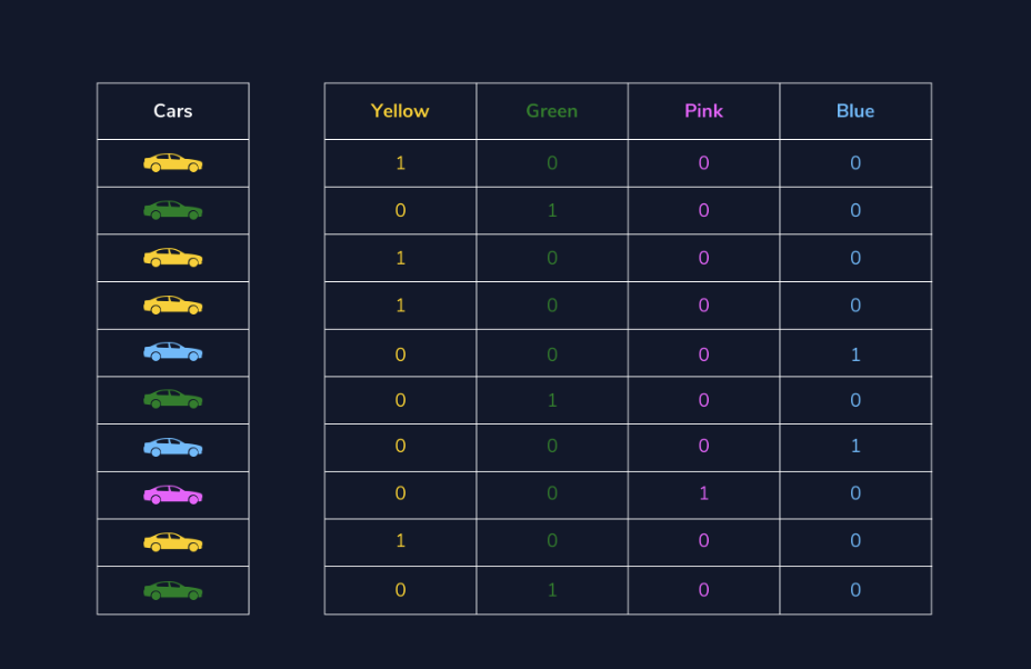
One-hot Encoding

One-hot encoding is when we create a dummy variable for each value of our categorical feature, and a dummy variable is defined as a numeric variable with two values: 1 and 0. We will continue to talk about color feature from the cars data frame.

Looking at this visual below, we can see we have ten cars in four different colors. In place of the single color column, we create four dummy variables - one new column for each color. Then the values that go into that column are binary, indicating if the car in that row is the color of the column name (1) or not (0).

import pandas as pd
# use pandas .get_dummies method to create one new column for each color
ohe = pd.get_dummies(cars['color'])

# join the new columns back onto our cars dataframe
cars = cars.join(ohe)

Binary encoding

If we find the need to one-hot encode a lot of categorical features which would, in turn, create a sparse matrix and may cause problems for our model, a strong alternative to this issue is performing a binary encoder. A binary encoder will find the number of unique categories and then convert each category to its binary representation.

To make this happen with Python we’ll use a library called category_encoders and import BinaryEncoder. We will determine which column to transform and set drop_invariant to True so it will keep the five binary columns. If it is set to the default 0, then we would have an additional column full of zeros.

from category_encoders import BinaryEncoder

#this will create a new data frame with the color column removed and replaced with our 5 new binary feature columns
colors = BinaryEncoder(cols = ['color'], drop_invariant = True).fit_transform(cars)

Hashing

Another option we have available to us is an encoding technique called hashing. This process is similar to one-hot encoding where it will create new binary columns, but within the parameters, you can decide how many features to output. A huge advantage is reduced dimensionality, but a large disadvantage is that some categories will be mapped to the same values. That is called collision.

For example, we have 19 different colored cars. If I were to use the hash encoder and set the number of features to be 5, I will definitely have a few colors with the same hash values.

from category_encoders import HashingEncoder

# instantiate our encoder
encoder = HashingEncoder(cols='color', n_components=5)

# do a fit transform on our color column and set to a new variable
hash_results = encoder.fit_transform(cars['color'])

Target encoding

Target encoding is a Bayesian encoder used to transform categorical features into hashed numerical values and is sometimes called the mean encoder. This encoder can be utilized for data sets that are being prepared for regression-based supervised learning, as it needs to take into consideration the mean of the target variable and its correlation between each individual category of our feature. In fact, the numerical values of each category is replaced with a blend of the posterior probability of the target given a particular categorical value and the prior probability of the target over all the training data.

Woah, now that was a lot of Bayesian buzzwords. How would it work with our specific color feature? It replaces each color with a blend of the mean price of that car color and the mean price of all the cars. Had it been predicting something categorical, it would’ve used a Bayesian target statistic.

Say we are preparing our dataset for a regression-based supervised learning algorithm that is trying to predict the selling price.

from category_encoders import TargetEncoder

# instantiate our encoder
encoder = TargetEncoder(cols = 'color')

# set the results of our fit_transform to a variable
# the output will be its own pandas series
encoder_results = encoder.fit_transform(cars['color'], cars['sellingprice'])

print(encoder_results.head())
#   color
# 0 11761.881473
# 1 18007.276995
# 2 8458.251232
# 3 14769.292595
# 4 12691.099747

We can examine all the different values our encoder_results holds, and if we look at the output from below we can see our min is about 3,054 and our max is about 18,048. That is quite a big difference!

# print all 19 unique values
print(np.sort(encoder_results['color'].unique()))
# OUTPUT
# [ 3054.12209927  8088.87434555  8458.25123153  9276.78571429
#   9867.50002121  9885.8093167  11043.90243902 11247.82608763
#  11761.88147296 11805.06187625 12124.83443709 12376.19047882
#  12691.09974747 13912.83399734 14769.29259451 15496.72704715
#  17174.36440678 17176.25931731 18007.27699531 18048.52540833]

Encoding date-time variable

Every data analyst or scientist will have to work with date-time objects at some point in their career. There is so much information to be gained from date-time objects. We will work with the saledate feature - yay, a new column to explore! The very first thing we need to do is convert this to a date-time object.

print(cars['saledate'].dtypes)
# # OUTPUT
# dtype('O')

cars['saledate'] = pd.to_datetime(cars['saledate'])
# #OUTPUT
# datetime64[ns, tzlocal()]

Now that we have our feature set up as a datetime object, let’s demonstrate some methods we can utilize to get additional information.

# create new variable for month
cars['month'] = cars['saledate'].dt.month

# create new variable for day of the week
cars['dayofweek'] = cars['saledate'].dt.day

# create new variable for difference between cars model year and year sold
cars['yearbuild_sold'] = cars['saledate'].dt.year - cars['year']

Let's fight the example

You are a data scientist at a clothing company and are working with a data set of customer reviews. This dataset is originally from Kaggle and has a lot of potential for various machine learning purposes. You are tasked with transforming some of these features to make the data more useful for analysis. To do this, you will have time to practice the following:

• Transforming categorical data
• Scaling your data
• Working with date-time features

import pandas as pd
import numpy as np
from sklearn.preprocessing import StandardScaler

#import data
reviews = pd.read_csv("reviews.csv")

#print column names
reviews.info()


#print .info
print(reviews.info())


#look at the counts of recommended
print(reviews["recommended"].value_counts())


#create binary dictionary
binary_dict = {True: 1, False: 0}

#transform column
reviews["recommended"] = reviews["recommended"].map(binary_dict)

#print your transformed column
print(reviews.head())

#look at the counts of rating
print(reviews["rating"].value_counts())

#create dictionary
rating_dict = {"Love it": 5, "Liked it": 4, "Was okay": 3, "Not great": 2, "Hated it": 1}


#transform rating column
reviews["rating"] = reviews["rating"].map(rating_dict)


#print your transformed column values
print(reviews["rating"].value_counts())

#get the number of categories in a feature
one_hot = pd.get_dummies(reviews["rating"])

#join the new columns back onto the original
reviews = reviews.join(one_hot)

#print column names
print(reviews.columns)