Why is this important?

Vectors and matrices are fundamental building blocks of data science as they are used to organize and manipulate data we feed through learning models. Whether you are just starting your journey in data science or have already played around with machine learning models, learning linear algebra fundamentals is key to your success in understanding advanced data science material.

There are many real-world applications of linear algebra, some of which we will cover in the coming exercises and lessons, including:

• Efficient computation of linear transformation on large quantities of data. Computer programs and hardware like GPUs have been optimized around these linear algebra data structures to enable much of the high-performance computing advances.

• Computer graphics, especially video games, rely heavily on linear algebra to render images quickly and efficiently.

• Machine learning and advances in deep learning, whose foundations are matrix and vector multiplication and addition.

What is Linear Algebra?

Linear algebra focuses on the mathematics surrounding linear operations and solving systems of linear equations. While most of us learned about basic linear operations in algebra classes in high school and middle school, linear algebra extends these lessons to apply to multi-dimensional data.

Linear algebra is fundamental because it allows us to mathematically operate on large amounts of data, which is vital to modern data science techniques. There are many real-world applications of linear algebra, some of which we will cover in the coming exercises and lessons, including:

• Solving systems of linear equations, especially those with many variables and cannot be reasonably solved by hand.

• Efficient computation of linear transformation on large quantities of data. Throughout this lesson, we will go into great detail on data structures that hold large amounts of data (vectors and matrices) and their various operations that allow us to apply linear transforms. Computer programs and hardware like GPU’s have been optimized around these linear algebra data structures to enable much of the high-performance computing advances.

• Computer graphics, especially video games, rely heavily on linear algebra to render images quickly and efficiently.

• Machine learning and advances in deep learning, whose foundations are matrix and vector multiplication and addition.

Vectors

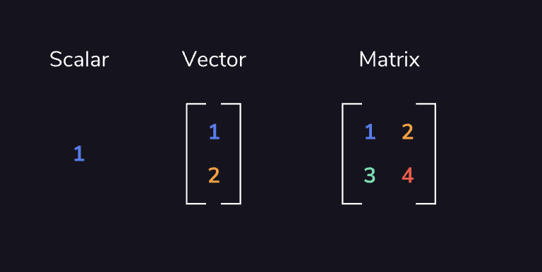
The fundamental building blocks of linear algebra are vectors. Vectors are defined as quantities having both direction and magnitude, compared to scalar quantities that have only magnitude, vector quantities consist of two or more elements of data.

The dimensionality of a vector is determined by the number of numerical elements in that vector.

# A 2-dimensional vector
v = [1, 2]

# A 3-dimensional vector
v = [1, 2, 3]

# A magnitude of a vector
import numpy as np

v = np.array([1, 2, 3])
magnitude = np.linalg.norm(v)
magnitude

Basic Vector operations

Scalar multiplication

Any vector can be multiplied by a scalar, which results in every element of that vector being multiplied by that scalar individually.

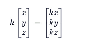
Multiplying vectors by scalars is an associative operation, meaning that rearranging the parentheses in the expression does not change the result. For example, we can say:

2(a3) = (2a)3.

Vectors can be added and subtracted from each other when they are of the same dimension (same number of components). Doing so adds or subtracts corresponding elements, resulting in a new vector of the same dimension as the two being summed or subtracted. Below is an example of three-dimensional vectors being added and subtracted together.

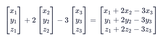
Vector addition is commutative, meaning the order of the terms does not matter. For example, we can say (a+b = b+a). Vector addition is also associative, meaning that (a + (b+c) = (a+b) + c).

Dot Product

An important vector operation in linear algebra is the dot product. A dot product takes two equal dimension vectors and returns a single scalar value by summing the products of the vectors’ corresponding components. This can be written out formulaically as:

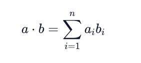
The dot product operation is both commutative (a · b = b · a) and distributive (a · (b+c) = a · b + a · c).

The resulting scalar value represents how much one vector “goes into” the other vector. If two vectors are perpendicular (or orthogonal), their dot product is equal to 0, as neither vector “goes into the other.”

Let’s take a look at an example dot product. Consider the following two vectors:

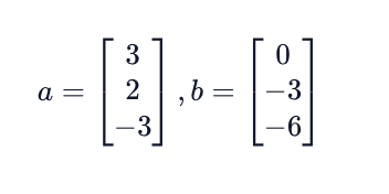
To find the dot product between these two vectors, we do the following:

Matrices

A matrix is a quantity with m rows and n columns of data. For example, we can combine multiple vectors into a matrix where each column of that matrix is one of the vectors.

We can think of vectors as single-column matrices in their own right.

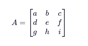
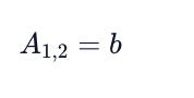
Matrices can be represented by using square brackets that enclose the rows and columns of data (elements). The shape of a matrix is said to be mxn, where m is the number of rows and n is the number of columns. When representing matrices as a variable, we denote the matrix with a capital letter and a particular matrix element as the matrix variable with an “m,n” determined by the element’s location.

The value corresponding to the first row and second column is b.

Matrix operations

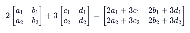
Like with vectors, there are fundamental operations we can perform on matrices that enable the linear transformations needed for linear algebra. We can again both multiply entire matrices by a scalar value, as well as add or subtract matrices with equal shapes.

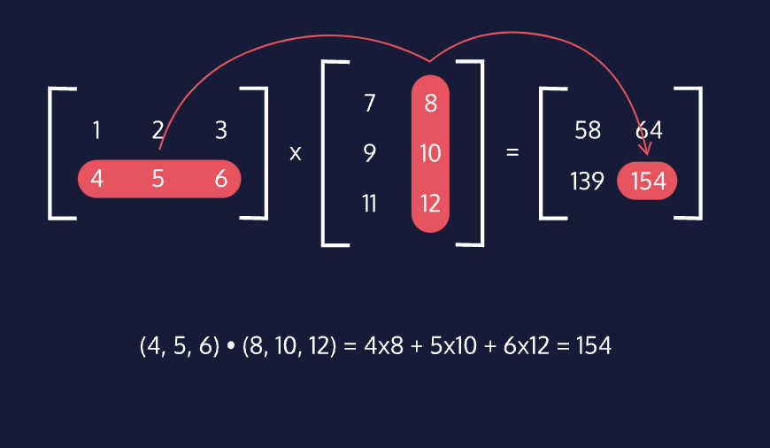
A new and important operation we can now perform is matrix multiplication. Matrix multiplication works by computing the dot product between each row of the first matrix and each column of the second matrix. For example, in computing AB = C, element (1,2) of the matrix product C will be the dot product of row 1 of matrix A and column 2 of matrix B.

An important rule about matrix multiplication is that the shapes of the two matrices AB must be such that the number of columns in A is equal to the number of rows in B. With this condition satisfied, the resulting matrix product will be the shape of rowsA x columnsB. For example, in the animation to the right, the product of a 2x3 matrix and a 3x2 matrix ends up being a 2x2 matrix.

Based on how we compute the product matrix with dot products and the importance of having correctly shaped matrices, we can see that matrix multiplication is not commutative, AB ≠ BA. However, we can also see that matrix multiplication is associative, A(BC) = (AB)C.

Special Matrices

There are a couple of important matrices that are worth discussing on their own.

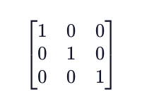
IDENTITY MATRIX

The identity matrix is a square matrix of elements equal to 0 except for the elements along the diagonal that are equal to 1. Any matrix multiplied by the identity matrix, either on the left or right side, will be equal to itself.

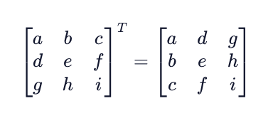
TRANSPOSE MATRIX

The transpose of a matrix is computed by swapping the rows and columns of a matrix. The transpose operation is denoted by a superscript uppercase “T” (AT).

PERMUTATION MATRIX

A permutation matrix is a square matrix that allows us to flip rows and columns of a separate matrix. Similar to the identity matrix, a permutation matrix is made of elements equal to 0, except for one element in each row or column that is equal to 1. In order to flip rows in matrix A, we multiply a permutation matrix P on the left (PA). To flip columns, we multiply a permutation matrix P on the right (AP).

Linear Systems in Matrix Form

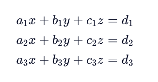
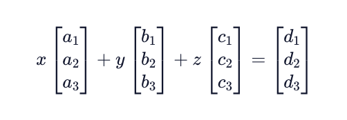
An extremely useful application of matrices is for solving systems of linear equations. Consider the following system of equations in its algebraic form.

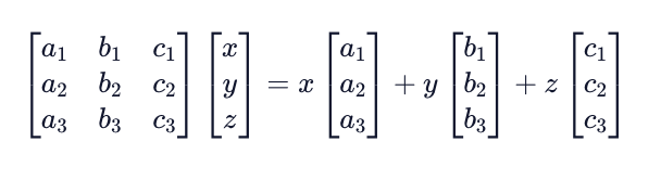
This system of equations can be represented using vectors and their linear combination operations that we discussed in the previous exercise. We combine the coefficients of the same unknown variables, as well as the equation solutions, into vectors. These vectors are then scalar multiplied by their unknown variable and summed.

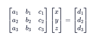
Our final goal is going to be to represent this system in form Ax = b, using matrices and vectors. As we learned earlier, we can combine vectors to create a matrix, which we will do with the coefficient vectors to create matrix A. We can also convert the unknown variables into vector x. We end up with the following Ax = b form:

Gauss-Jordan Elimination

Now that we have our system of linear equations in augmented matrix form, we can solve for the unknown variables using a technique called Gauss-Jordan Elimination. In regular algebra, we may try to solve the system by combining equations to eliminate variables until we can solve for a single one. Having one variable solved for then allows us to solve for a second variable, and we can continue that process until all variables are solved for.

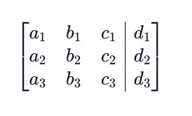
The same goal can be used for solving for the unknown variables when in the matrix representation. We start with forming our augmented matrix.

To solve for the system, we want to put our augmented matrix into something called row echelon form where all elements below the diagonal are equal to zero. This looks like the following:

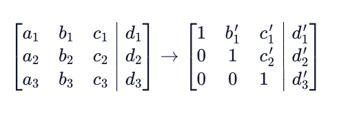
Note that the values with apostrophes in the row echelon form matrix mean that they have been changed in the process of updating the matrix. Once in this form we can rewrite our original equation as:

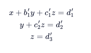
This allows us to solve the equations directly using simple algebra. But how do we get to this form?

To get to row echelon form we swap rows and/or add or subtract rows against other rows. A typical strategy is to add or subtract row 1 against all rows below in order to make all elements in column 1 equal to 0 under the diagonal. Once this is achieved, we can do the same with row 2 and all rows below to make all elements below the diagonal in column 2 equal to 0.

Once all elements below the diagonal are equal to 0, we can simply solve for the variable values, starting at the bottom of the matrix and working our way up.

It’s important to realize that not all systems of equations are solvable! For example, we can perform Gauss-Jordan Elimination and end up with the following augmented matrix.

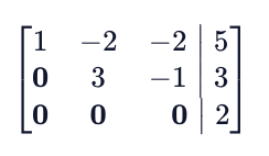
This final augmented matrix here suggests that 0z = 2, which is impossible!

One more time

Imagine we have the following system of linear equations:

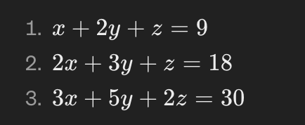
Step 1: Form the Augmented Matrix First, we write this system as an augmented matrix, combining the coefficients of the variables and the constants into one matrix:

Step 2: Obtain Leading Ones

We want a leading 1 in the first row, first column. It's already there, so no row operation is needed for this step.

Step 3: Zero Out Below the Pivot

Use row operations to make the entries below this leading 1 into 0s. For our matrix:

• Subtract 2 times the first row from the second row.
• Subtract 3 times the first row from the third row.

Step 4: Move to the Next Pivot

Move to the second row, second column. Make this a 1 (if it's not already) by dividing the whole row by the coefficient of y in this row. Then, use row operations to make all other entries in this column 0.

Step 5: Repeat the Remaining Columns

Continue this process for the third column. You'll aim to have a leading 1 in the third row, third column, and zeros everywhere else in this column.

Step 6: Achieve Reduced Row Echelon Form (RREF)

After completing these steps, the matrix will be in RREF. In our example, the final matrix might look something like this (note, the exact numbers here are for illustrative purposes and may not match the actual outcomes of the operations described):

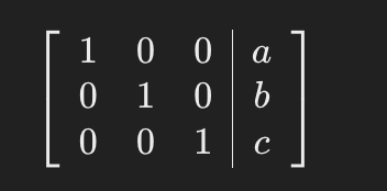
Where a, b, and c are the solutions to the system of equations for x, y, and z, respectively.

CONCLUSION

Each row of the matrix now corresponds to an equation where one of the variables equals a number. In this simplified form, the solution to the system of equations can be read directly: x = a, y = b, and z = c.

This method systematically eliminates variables from the equations by transforming the matrix, making it easier to solve complex systems of equations. It might seem a bit abstract at first, but with practice, it becomes a powerful tool for solving linear algebra problems.