Introduction

Feature engineering is an integral part of building and implementing machine learning models. In this article, you’ll learn about what feature engineering is, why we need it and where it fits in within the machine learning workflow. Additionally, you’ll get a brief overview of the many data science tools involved in feature engineering and how they assist data scientists in model diagnostics.

What is Feature Engineering?

A feature is a measurable property in a dataset, and a feature can be used as an input to a machine learning model. One way to think about features is as predictor variables that go into a model to predict the outcome variable.

Often, when presented with a dataset, it might not be clear what features we should use for a specific model (i.e., should we use ‘tree density’ as an input to our precipitation model?). Similarly, in large datasets, there might be too many features to manually decide which features to use. Some features might be highly correlated with one another, some might not vary much with the outcome variable, and some might be in the wrong form to be a model input and so on. It is not uncommon that a data scientist might not realize any of this until they begin diagnosing a model that is performing poorly.

Feature engineering is the process of transforming raw data into features that better represent the underlying problem to the predictive models, resulting in improved model accuracy on unseen data. It is the process of selecting, creating, and transforming features to improve the performance of a model.

Why is Feature Engineering Important?

1. Performance

We would like our machine learning model to perform well on our data. If it is not able to predict the outcome variable (to a reasonable degree of accuracy) on known data, it would be unwise to use it to predict outcomes on unknown data.

2. Runtime

Suppose a model has excellent performance but takes a really long time to run. For a data scientist, depending on their available computational resources, such a model might be impractical for production.

3. Interpretability

A model is only as good as the insights it helps us glean from the data. Data scientists are often tasked with finding out what factors drive different outcomes. A well-performing model would not be of much help if it’s opaque and uninterpretable.

4. Generalizability

We would like our model to generalize well to unseen data. Often data scientists work with streaming data and need their model to be flexible with new and unknown data..

Feature Engineering and the Machine Learning workflow

So where does feature engineering fall within the machine learning workflow?

Feature engineering is ofen introduced as an intermediate step between exploratory data analysis and implementing a machine learning algorithm. In reality, these distinctions are fuzzy and the process is not exactly linear.

Broadly, we can divide feature engineering techniques into three categories:

1. Feature Transformation methods:

These involve numerical transformations methods and ways to encode non-numerical variables. These techniques are applied before implementing a machine learning model. They include and are not limited to: scaling, binning, logarithmic transformations, hashing and one hot encoding. These methods typically improve performance, runtime and interpretability of a model.

2. Dimensionality Reduction methods:

Dimensionality of a dataset refers to the number of features within a dataset and reducing dimensionality allows for faster runtimes and (often) better performance. This is an extremely powerful tool in working with datasets with “high dimensionality”. For instance, a hundred-feature problem can be reduced to less than ten modified features, saving a lot of computational time and resources while maintaining or even improving performance. Typically, dimensionality reduction methods are machine learning algorithms themselves, such as Principal Component Analysis (PCA), Linear Discriminant Analysis (LDA), etc.

3. Feature Selection methods:

Feature selection methods are a set of techniques that allow us to choose among the pool of features available. Unlike dimensionality reduction, these retain the features as they are which makes them highly interpretable. They usually belong to one of these three categories:

I. Filter methods:

These are statistical techniques used to filter out usefule features. Filter methods are completely model agnostic (the can be used with any model) and are useful sanity checks for a data scientist to carry out before deciding on a model. They include and are not limited to: correlation coefficients (Pearson, Spearman, etc.), mutual information, chi-squared, ANOVA, etc.

II. Wrapper methods:

Wrapper methods search for the best set of features by using a greedy search strategy. They pick a subset of features, train a model, evaluate it, try a different subset of features, train a model again, and so on until the best possible set of features and most optimal performance is reached. As this could potentially go on forever, a stopping criterion based on number of features or a model performance metric is typically used. Forward Feature Selection, Backward Feature Elimination and Sequential Floating are some examples of wrapper method algorithms.

III. Embedded methods:

Embedded methods are implemented during the model implementation step. Regularization techniques such as Lasso or Ridge tweak the model to get it to generalize better to new and unknown data. Tree-based feature importance is another widely used embedded method. This method provides insight into the features that are most relevant to the outcome variable while fitting decision trees to the data.

Data centering

Data centering involves subtracting the mean of a data set from each data point so that the new mean is 0. This process helps us understand how far above or below each of our data points is from the mean.

#get the mean of your feature
mean_dis = np.mean(distance)

#take our distance array and subtract the mean_dis, this will create a new series with the results
centered_dis = distance - mean_dis

#visualize your new list
plt.hist(centered_dis, bins = 5, color = 'g')

#label our visual
plt.title('Starbucks Distance Data Centered')
plt.xlabel('Distance from Mean')
plt.ylabel('Count')
plt.show()

Standardizing Data

Standardization (also known as Z-Score normalization) is when we center our data, then divide it by the standard deviation. Once we do that, our entire data set will have a mean of zero and a standard deviation of one. This allows all of our features to be on the same scale. How cool is that?

This step is critical because some machine learning models will treat all features equally regardless of their scale. You’ll definitely want to standardize your data in the following situations:

• Before Principal Component Analysis (PCA)
• Before using any clustering or distance based algorithms (K-Means, K-Nearest Neighbors, etc.)
• Before KNN
• Before using any regularization techniques (Lasso, Ridge, etc.)

import pandas as pd
import numpy as np

coffee = pd.read_csv('starbucks_customers.csv')
ages = coffee['age']

## add code below
## set up your variables

mean_age = np.mean(ages)
std_dev_age = np.std(ages)

## standardize ages
ages_standardized = (ages - mean_age)/std_dev_age


## print the results

print(np.mean(ages_standardized))
print(np.std(ages_standardized))

Min-Max normalization

Another form of scaling your data is to use Min-Max normalization process. The name says it all, we find the minimum and maximum data point in our entire data set and set each of those to 0 and 1, respectively.

Then the rest of the data points will transform to a number between 0 and 1, depending on its distance between the minimum and maximum number. We find that transformed number by taking the data point subtracking it from the minimum point, then dividing by the value of our maximum minus minimum.

Mathematically a min-max normalization looks like this:

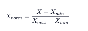
One thing to note about min-max normalization is that this transformation does not work well with data that has extreme outliers. You will want to perform a min-max normalization if the range between your min and max point is not too drastic.

The reason we would want to normalize our data is very similar to why we would want to standardize our data - getting everything on the same scale.

import pandas as pd
import numpy as np

coffee = pd.read_csv('starbucks_customers.csv')

## add code below
## get spent feature

spent = coffee["spent"]

#find the max spent
max_spent = np.max(spent)

#find the min spent
min_spent = np.min(spent)

#find the difference
spent_range = max_spent - min_spent

#normalize your spent feature
spent_normalized = (spent - min_spent)/spent_range

#print your results
print(spent_normalized)

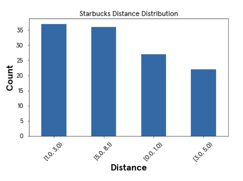
Binning Data

Binning data is the process of taking numerical or categorical data and breaking it up into groups. We could decide to bin our data to help capture patterns in noisy data. There isn't a clean and fast rule about how to bin your data, but like so many things in machine learning, you need to be aware of the trade-offs.

You want to make sure that your bin ranges aren’t so small that your model is still seeing it as noisy data. Then you also want to make sure that the bin ranges are not so large that your model is unable to pick up on any pattern. It is a delicate decision to make and will depend on the data you are working with.

import pandas as pd
import numpy as np
import matplotlib.pyplot as plt
import codecademylib3_seaborn

coffee = pd.read_csv('starbucks_customers.csv')
ages = coffee['age']

print(np.min(ages))
print(np.max(ages))

age_bins=[12, 20, 30, 40, 71]

coffee["binned_ages"] = pd.cut(coffee['age'], age_bins, right=False)

print(coffee["binned_ages"].head(10))
coffee["binned_ages"].value_counts().plot(kind="bar")
plt.show()