Inferential Statistics

Descriptive statistics and inferential statistics are two subfields of statistics. Descriptive statistics includes topics covered earlier in this path, including numerical and visual summaries of data. Hypothesis testing, on the other hand, is a form of inferential statistics, which is used to draw inferences about a population using a smaller sample of data.

Descriptive statistics tells us about the data that we have, but sometimes we can't collect all of the data that we need to answer our questions.

For example, maybe we want to know whether people who get a vaccine are less likely to get a disease. We can’t vaccinate every single person in the world to test this, so we’ll have to vaccinate a smaller sample of people instead. Then, if the vaccine seems to work in our sample, we need to know whether that could have been a random fluke — or if it’s likely to be true for the rest of the population. This is where hypothesis testing can help.

Inferential statistics is all about using a sample (a subset of population) to make inferences about a larger population of interests. This is useful when we want to know something about a population but cannot observe every member - often due to time, feasibility, or monetary constraints.

Some methods that are used in inferential statistics include hypothesis testing, confidence intervals, and regression analysis.

Introduction to Hypothesis Testing

Hypothesis testing is a framework for asking questions about a dataset and answering them with probabilistic statements.

There are many different kinds of hypothesis tests that can be used to address different kinds of questions and data.

Example

STEP 1 - Ask a question

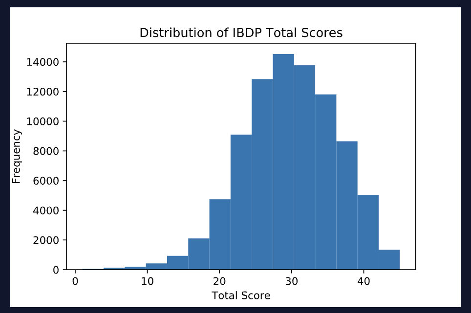
The International Baccalaureate Degree Programme (IBDP) is a world-wide educational program. Each year, students in participating schools can take a standardized assessment to earn their degree. Total scores on this assessment range from 1-45. Based on data provided here, the average total score for all students who took this exam in May 2020 was around 29.92. The distribution of scores looks something like this:

Imagine a hypothetical online school, Statistics Academy, that offers a 5-week test-preparation program. Suppose that 100 students who took the IBDP assessment in May 2020 were randomly chosen to participate in the first group of this program and that these 100 students earned an average score of 31.16 points on the exam — about 1.24 points higher than the international average.

Are these students really outperforming their peers? Or could this difference be attributed to random chance?

STEP 2 - Define the Null and Alternative Hypotheses

Before attempting to answer this question, it is useful to reframe it in a way that is testable. Right now, our question (“Are the Statistics Academy students really outperforming their peers?”) is not clearly defined. Objectively, this group of 100 students performed better than the general population — but answering “yes, they outperformed their peers!” doesn’t feel particularly satisfying.

The reason it's not satisfying is this: if we randomly choose ANY group of 100 students from the population of all test takers and calculate the average score for that sample, there is a 50% chance it will be higher than the population average. Observing a higher average for a single sample is not surprising.

Of course, large differences from the population average are less probable — if all the Statistics Academy students earned 45 points on the exam (the highest possible score), we’d probably be convinced that these students had a real advantage. The trick is to quantify when differences are “large enough” to convince us that these students are systematically different from the general population. We can do this by reframing our question to focus on population(s), rather than our specific sample(s).

A hypthesis test begins with two competing hypotheses about the population that a particular sample comes from - in this case, the 100 Statistics Academy students:

• Hypothesis 1 (the Null Hypothesis): The 100 Statistics Academy students are a random sample from the general population of test takers, who had an average score of 29.92. If this hypothesis is true, the Statistics Academy students earned a slightly higher average score by random chance.

• Hypothesis 2 (the Alternative Hypothesis): The 100 Statistics Academy students came from a population with an average score that is different from 29.92. In this hypothesis, we need to imagine two different populations that don’t actually exist: one where all students took the Statistics Academy test-prep program and one where none of the students took the program. If the alternative hypothesis is true, our sample of 100 Statistics Academy students came from a different population than the other test-takers.

There’s one more clarification we need to make in order to fully specify the alternative hypothesis. Notice that, so far, we have not said anything about the average score for “population 1” in the diagram above, other than that it is NOT 29.92. We actually have three choices for what the alternative hypothesis says about this population average:

• it is GREATER THAN 29.92
• it is NOT EQUAL TO (i.e., GREATER THAN OR LESS THAN) 29.92
• it is LESS THAN 29.92

STEP 3 - Determine the Null Distribution

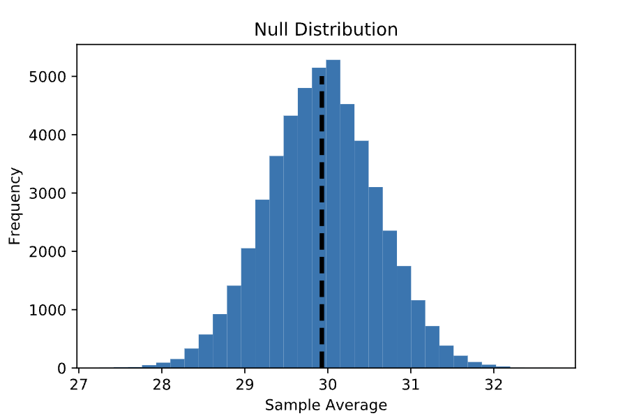
Now that we have our null hypothesis, we can generate a null distribution: the distribution (across repeated samples) of the statistic we are interested in if the null hypothesis is true. In the IBDP example described above, this is the distribution of average scores for repeated samples of size 100 drawn from a population with an average score of 29.92.

Statistical theory allows us to estimate the shape of this distribution using a single sample. You can learn how to do this by reading more about the CLT, but for the purposes of this example, let’s simulate the null distribution using our population. We can do this by:

• Taking many random samples of 100 scores, each, from the population

• Calculating and storing the average score for each of those samples

• Plotting a histogram of the average scores

This yields the following distribution, which is approximately normal and centered at the population average:

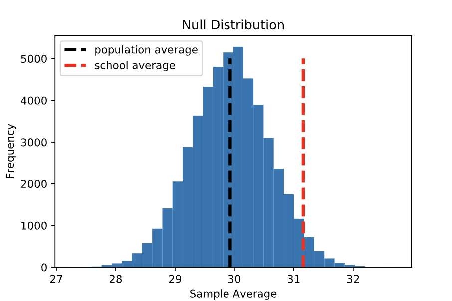
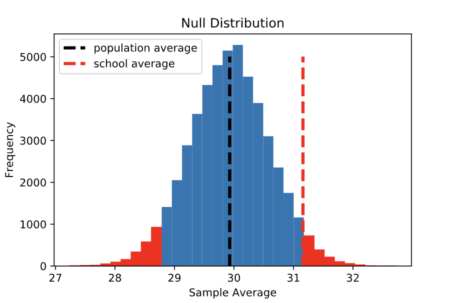
If the null hypothesis is true, then the average score of 31.16 observed among Statistics Academy students is simply one of the values from this distribution. Let’s plot the sample average on the null distribution. Notice that this value is within the range of the null distribution, but it is off to the right where there is less density:

STEP 4 - Calculate the p-value (or confidence interval)

Here is the basic question asked in our hypothesis test:

Given that the null hypothesis is true (that the 100 students from Statistics Academy were sampled from a population with an average IBDP score of 29.92), how likely is it that their average score is 31.16?

The minor problem with this question is that the probability of any exact average score is very small, so we really want to estimate the probability of a range of scores. Let’s now return to our three possible alternative hypotheses and see how the question and calculation each change slightly, depending on which one we choose:

OPTION 1

Alternative Hypothesis: The sample of 100 scores earned by Statistics Academy students came from a population with an average score that is greater than 29.92.

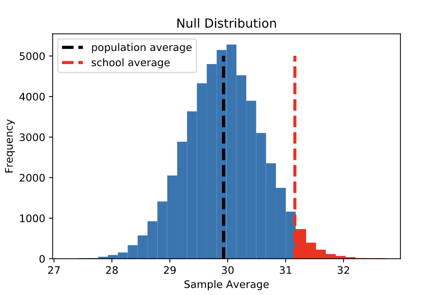
In this case, we want to know the probability of observing a sample average greater than or equal to 31.16 given that the null hypothesis is true. Visually, this is the proportion of the null distribution that is greater than or equal to 31.16 (shaded in red below). Here, the red region makes up about 3.1% of the total distribution. This proportion, which is usually written in decimal form (i.e., 0.031), is called a p-value.

OPTION 2

Alternative Hypothesis: The sample of 100 scores earned by Statistics Academy students came from a population with an average score that is not equal to (i.e., greater than OR less than) 29.92.

We observed a sample average of 31.16 among the Statistics Academy students, which is 1.24 points higher than the population average (if the null hypothesis is true) of 29.92. In the first version of the hypothesis test (option 1), we estimated the probability of observing a sample average that is at least 1.24 points higher than the population average. For the alternative hypothesis described in option 2, we’re interested in the probability of observing a sample average that is at least 1.24 points DIFFERENT (higher OR lower) than the population average. Visually, this is the proportion of the null distribution that is at least 1.24 units away from the population average (shaded in red below). Note that this area is twice as large as in the previous example, leading to a p-value that is also twice as large: 0.062.

While option 1 is often referred to as a One Sided or One-Tailed test, this version is referred to as a Two Sided or Two-Tailed test, referencing the two tails of the null distribution that are counted in the p-value. It is important to note that most hypothesis testing functions in Python and R implement a two-tailed test by default.

OPTION 3

Alternative Hypothesis: The sample of 100 scores earned by Statistics Academy students came from a population with an average score that is less than 29.92.

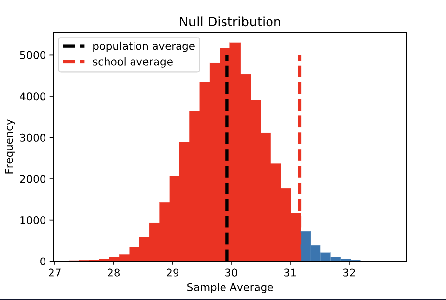
Here, we want to know the probability of observing a sample average less than or equal to 31.16, given that the null hypothesis is true. This is also a one-sided test, just the opposite side from option 1. Visually, this is the proportion of the null distribution that is less than or equal to 31.16. This is a very large area (almost 97% of the distribution!), leading to a p-value of 0.969.

At this point, you may be thinking: why would anyone ever choose this version of the alternative hypothesis?! In real life, if a test-prep program was planning to run a rigorous experiment to see whether their students are scoring differently than the general population, they should choose the alternative hypothesis before collecting any data. At that point, they won’t know whether their sample of students will have an average score that is higher or lower than the population average — although they probably hope that it is higher.

STEP 5 - Interpret the results

In the three examples above, we calculated three different p-values (0.031, 0.062, and 0.969, respectively). Consider the first p-value of 0.031. The interpretation of this number is as follows:

If the 100 students at Statistics Academy were randomly selected from the full population (which had an average score of 29.92), there is a 3.1% chance of their average score being 31.16 points or higher.

This means that it is relatively unlikely, but not impossible, that the Statistics Academy students scored higher (on average) than their peers by random chance, despite no real difference at the population level. In other words, the observed data is unlikely if the null hypothesis is true. Note that we have directly tested the null hypothesis, but not the alternative hypothesis! We therefore need to be a little careful about how we interpret this test: we cannot say that we’ve proved that the alternative hypothesis is the truth — only that the data we collected would be unlikely under null hypothesis, and therefore we believe that the alternative hypothesis is more consistent with our observations.